Causal Inference - To Control or not to Control

I will avoid repeating most of the stuff that can be found in other tutorials and books e.g. what is a collider or fork. I will provide useful links when a relevant topic is discussed. Otherwise, I assume that the reader is either familiar with the topic or sufficiently motivated to learn more. Just in case you feel lack of knowledge or context, here is a set of resources I would recommend to consult with:
[ Introductory course on Causal Inference, Causal Inference: The Mixtape Causal Inference in Statistics: A Primer, Causality ]

As the first experiment to my writing I chose to write about causal inference and also conduct a small exercise based on this paper. This paper is discussed in the forth week of Introductory course on Causal Inference.
The difference here is that I kept:

1. the relationship between variables exactly the same, while in the video they were modified
2. the treatment variable continuous, while in the video it was modified to a binary variable in order to show one particular technique of estimating the average treatment effect.

Also, I am willing to connect some dots on why certain techniques are working on estimating average causal effect and highlight what happens if proceed in estimating the causal effect naively.

“My mama always said life was like a box of chocolates. You never know what you’re gonna get” © - Forrest Gump

Causal Inference … where is it needed?
Short: When Randomized Controlled Trials (RCTs) are not possible. There are plenty reasons why it would not be possible to conduct a RCT, some of them are described in the “Why CI in industry” subsection of the referred blog-post.

To motivate our exercise, let us imagine the following situation:
You are chilling at work, mangling with the data or playing a stare contest with the Tensorboard, when your boss calls you and asks you to look into the effect of variable $X$ on the business KPI $Y$.

What would be your possible answer?

A. Well to precisely understand the effect we need to setup a RCT, turn off the product feature $X$ for some percentage of users for N amount of time.

B. Okay, I will do what I can.

In case you answer A it leads to a lot of complications:

1. It might be that feature $X$ is a successful one: turning it off can result in a lot of opportunity cost

2. RCT? Easier said than done. Setting up RCT has its own challenges. Even companies with mature A/B testing frameworks struggle to get it right sometimes.

3. What if what you’re trying to randomize is not possible to randomize?

Outcome: if your intention was that your boss buggers off, well, mission accomplished!

In case your answer is B, then I hope the exercise below will shed some light on some practical and also theoretical questions. More specifically:

• How/Why linear regression coefficients can be used to estimate average causal effect of one variable on another?
• What happens if wrong variables are controlled during the estimation of average causal effect?

A bit about Data Generation Process

When we talk about data generation process, we have to talk about its causal structure. To represent the causal structure of the world, current literature suggests two instruments:

1. Structural Causal Models (SCM)
2. Graphical Models

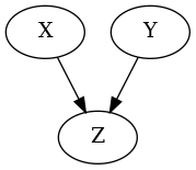
Given random variables $X$, $Y$ and $Z$, SCM could be $Z=f(X, Y)$. Which means that variables $X$ and $Y$ are causing the variable $Z$. Also, the part of the SCM is to describe the exact form of the $f$. It is often a convenient choice to model the relationship between variables as linear functions (the reason $\rightarrow$ interpretability).

Example: $f_{Z}: Z = 2X + \frac{Y}{5} + \epsilon$.

The graphical model corresponding to the SCM above would look like this:

To follow the data generation process offered in the paper I did two things. Translated the witchcraft written in R (no offense to R experts, I just detest that language) to Python and introduced a bit of structure to it:

• Variables
• SCM
• DataGenerator

In all studies presented in the paper, the effect of variable $T$ to $Y$ is always the subject of study. Therefore when talking about particular structures like forks or colliders it is meant to highlight how the 3rd variable is related to $T$ and $Y$.

Generating a Fork Structure

W = Variable('W', EXOGENOUS_TYPE)
T = Variable('T', ENDOGENOUS_TYPE)
Y = Variable('Y', ENDOGENOUS_TYPE)

fork_scm = SCM("Fork")

fork_scm.add_equation(W, {})
fork_scm.add_equation(outcome_variable=T, input_variables={W: 0.5})
fork_scm.add_equation(outcome_variable=Y, input_variables={W: 0.4, T: 0.3})

fork_data = SimpleDataGenerator().generate(fork_scm, 1000, 777)

With corresponding SCM and graphical model:

\(f_{T}: T = 0.5W\)
\(f_{Y}: Y = 0.4W + 0.3T\)

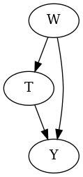
Two more examples can be found here in this notebook. In all of them the average causal effect ($ACE$: vocabulary borrowed from Judea Pearl) of $T$ on $Y$ is studied. In other literature $ACE$ is named as $ATE$ (average treatment effect). Personally I like average causal effect as average treatment effect suggest binarization of variable T. E.g. whether subjects they were treated or not. These are just semantics. Maybe it’s just me :)

To understand the procedure of estimating the $ACE$, let us do one step back.

A bit of formalism: A little tale about Regression coefficients

For a second lets imagine that:

and we fit a linear regression to satisfy

where $X$ is a vector of other covariates. Let us rewrite $\hat{Y}$ in terms of expected values:

And for every $value$ of $T$:

Now let us see what happens with difference of expected values when we change the $value$ by $\delta$. $\delta$ represents a unit change in the value of $T$. Without loss of generality we can assume that $\delta = 1$.

Which should not come to a surprise to us: this is how we usually interpret coefficients of linear regression - as expected change in the outcome variable when the respective covariate is changed by one unit. However, is this estimate truly carries a causal nature? Let us do one more step to understand the difference.

A bit more of formalism

In case $T$ is binary, we define $ACE$ as:

The important distinction between left and right sides of the $ =?$ sign is the presence of the $do$-operator. $do$-operator represents the intervention. More specifically, $E[Y|do(T=1)]$ measures the expected value of $Y$ when everyone in the population took the treatment $T$, while $E[Y|T=1]$ the expected value of $Y$ conditioned on the sub-population that took the treatment $T$.

Now when $T$ is a continuous value we are interested in:

As in case of linear regression, we can assume $\delta=1$. The left side of the above equation translates to:

“What is the average causal effect of the treatment variable $T$ on the outcome variable $Y$, when we change variable $T$ by one unit”

An important question here is “how can we express the left side of the =? in terms of the right side?”

Definition (The Backdoor Criterion): Given an ordered pair of variables $(T,Y)$ in a DAG $G$, a set of variables $Z$ satisfies the backdoor criterion relative to $(T, Y)$ if no node in $Z$ is descendant of $T$, and $Z$ blocks every path between $T$ and $Y$ that contains an arrow into $T$.

(above definition is taken from Judea Pearl)

Which basically means that in order to have the decomposition above, one needs to control for all variables that are not descendants of $T$ and should not control for any of descendants.

Well, let’s see how this relates to regression coefficients in case we have to control for only one variable $Z$:

Now, in case of linear relationship between variables:

And similarly to derivations for linear regression we can derive from just obtained results that:

Which basically shows in case we control for right variables, we can estimate the $ACE$ by fitting a linear regression (of course it is true only when SCM consists of linear relationships) to the data and look at the coefficient of the treatment variable.

Carrying out experiments

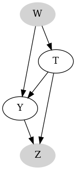
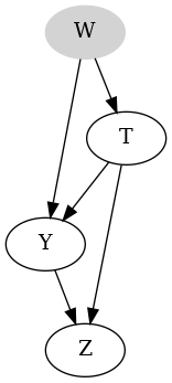
The paper simulates data over a realistic study over the relationship of 24-h dietary sodium intake ($T$) and systolic blood pressure ($Y$). With age $W$ our kidneys undergo transformations which effects the balance of sodium in our organism and systolic blood pressure. Thus, $W$ is a common cause of both $T$ and $Y$. On the other hand having 24-h dietary sodium intake and high systolic blood pressure both cause excretion of urinary protein $Z$. Thus, $Z$ is a caused both by $T$ and $Y$.

The data generation process and the resulting graph are depicted below:

Generating Fork + Collider Data

W = Variable('W', EXOGENOUS_TYPE, config={'mean': 65, 'std': 5}) # Age
T = Variable('T', ENDOGENOUS_TYPE)
Y = Variable('Y', ENDOGENOUS_TYPE)
Z = Variable('Z' , ENDOGENOUS_TYPE)

use_case_scm = SCM('UseCase')

use_case_scm.add_equation(W, {})
use_case_scm.add_equation(outcome_variable=T, input_variables={W: 0.056})
use_case_scm.add_equation(outcome_variable=Y, input_variables={T: 1.05, W: 2.0})
use_case_scm.add_equation(outcome_variable=Z, input_variables={Y: 2.0, T: 2.8})

use_case_data= SimpleDataGenerator().generate(use_case_scm, 1000, 777)

With corresponding SCM and graphical model:

\(f_{T}: T = 0.056W\)
\(f_{Y}: Y = 1.05T + 2.0W\)
\(f_{Z}: Z = 2.0Y + 2.8T\)

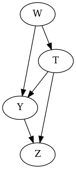
Here we can see that the causal effect of $T$ on $Y$ is $1.05$.

Assumptions

We assume that we have been provided with the graphical model and that we know that the relationship between variables is linear.

“How do we obtain such a graphical model in real world scenarios?” - Good question!

Here is how:

1. There is a branch of research devoted to learning the causal DAG from the data.
2. Domain knowledge: Given the data and sufficient expertise in the domain one can come up with a pretty decent graphical model.

Estimation

As was shown above, what we need is to fit a linear regression on a set of variables and look at the coefficient of the variable $T$.

Now let’s see how far we can get with different approaches of estimating the $ACE$…

Approach 1: Adjust for nothing

==============================================================================
                 coef    std err          t      P>|t|      [0.025      0.975]
------------------------------------------------------------------------------
const        122.4095      1.111    110.184      0.000     120.229     124.590
T            **3.2167**    0.292     11.029      0.000       2.644       3.789
==============================================================================

Here we just overestimated the effect of $T$ by $207$%. Imagine the implications on the business in case you communicated an estimate like this to your boss. Conclusion: just collecting the data and comparing group means without further checks is a NO-NO!.

Approach 2: Brutal Data Scientist mode - pour all variables in: adjust for both $W$ and $Z$

==============================================================================
                 coef    std err          t      P>|t|      [0.025      0.975]
------------------------------------------------------------------------------
const          0.2136      0.180      1.186      0.236      -0.140       0.567
T           **-0.9117**    0.033    -27.778      0.000      -0.976      -0.847
W              0.3961      0.024     16.208      0.000       0.348       0.444
Z              0.4002      0.006     65.525      0.000       0.388       0.412
==============================================================================

He? $-0.9117$ ? Completely different sign. Which means not only the magnitude is wrong but also conclusions are 180 degrees different.

In a simplified world, for the first approach you could communicate to your boss “if you spend one dollar, you will generate 3.22” In the second case the message would be “if you spend one dollar, you are going to lose additional 90 cents”.

Approach 3: we stop cutting corners and look at the DAG. The DAG says, $W$ is a fork and $Z$ is a collider. Or putting in Backdoor Criterion (BC) words, $Z$ does not satisfy BC criterion and $W$ does. Therefore we need to control only for $W$.

==============================================================================
                 coef    std err          t      P>|t|      [0.025      0.975]
------------------------------------------------------------------------------
const          0.8931      0.414      2.157      0.031       0.081       1.706
T            **1.0517**    0.031     34.101      0.000       0.991       1.112
W              1.9864      0.007    305.330      0.000       1.974       1.999
==============================================================================

Seems like we hit the target. One disturbing thing here is the width of the confidence interval. They look like Grond went through it.

But this is a story for another time….

If you’re reading this line it means you have made it through :)) Thanks for reading! I will come back to causal inference topic in the future to cover more realistic and interesting use-cases.